Homework 2
Additive / Navigational Potential Functions
Introduction
This report will cover implementation and observations of prominent robot motion algorithms. They are namely Simple Potential Field Planner and Navigational Function based Planer. respectively. Furthermore, in the discussion part there will be comparison of both algorithms in terms of performance and completeness.
In this homework we again assume a point robot to find complete path to the goal at time same time avoiding obstacles. Unlike the bug algorithms which works only 2D configuration space, here potential functions can be applied to more general class of configuration spaces.
Attractive/Repulsive Potential
Idea of potential functions is actually an energy function that can be differentiable. Therefore its derivative has a direction means force. By saying differentiable here in this context is gradient of the function. This energy function is similar to magnetic fields in physics.
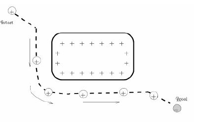
Figure 1-Potential Field
Left figure can represent this phenomena well. Robot can move under the effect of attractive and repulsive forces. This forces creates values that are high far from the goal and near obstacles and low nearby and on the robot. Gradient of those values move robot to the goal.
Important thing here that gradient is actually intentionally selected as velocity instead of force. Main idea for selecting like this is to ignore dynamic part of the algorithm. We want to pay attention to motion planning part more than to dynamic part. That part is actually topic of another field of the robotic world which is called Robot/Legged Locomotion. (see. web page).
Equation 1-Total potential formula
Actually attractive and repulsive fields can be depicted like this:
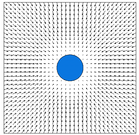
Attractive Potential Function
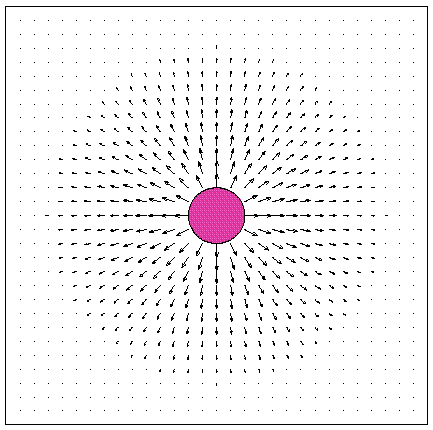
Repulsive Potential Function
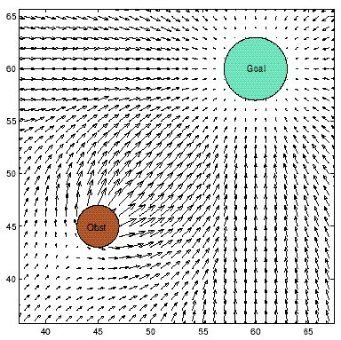
Vector Summation of Two Fields
Interactive Trial of Attractive and Repulsive Vectors
You can try and observe how simple potential function works. Green vector is always towards to the goal, Red vector is summation of repulsive vectors and finally Blue vector is the summation of attractive and repulsive vectors.
When you move the mouse cursor near to obstacles (closer than 100 px), dashed red line appears. This line says that robot at that location is under repulsive function. As you move closer you will observe that repulsive force increases dramatically, so the summation of two forces (shown as blue).
If no Blue vector occurs that mean we are on the local minima that means there is no motion vector and we are stuck. At this kind of points, attractive and repulsive vectors are the same with opposite direction.
Potential Fields on a Robot
You can go to Simple Potential Robot page to use interactive interface to experience simple potential fields on a point robot. You can drag and move the robot to anywhere in the free space. It is also possible to draw new obstacles and experience how robot attitude simultaneously.
Video 1-Robot can find its path using simple potential field
Easy Obstacle Configuration
We captured this simple potential field planner using our interactive potential field tool. If there is no obstacle goal point's attractive force can easily pull robot.
As you can realize, as robot approaches to obstacles (threshold value is 100px), there is no longer only attractive force, but repulsive forces also. Velocity of the robot is getting slower as repulsive force (shown as dashed red) occurs in the opposite direction of the attractive force (shown as dashed green).
Video 2-A little bit difficult path finding with new obstacles on robot's way
More Difficult Obstacle Configuration
However, if we have obstacles very close to robot's way things change. You will see that in the following example.
Using our interactive tool, we can insert new obstacles. Here we add some obstacles nearby robot's goal which are also on the possible path.
As you can realize, attractive force (shown as dashed green) is getting smaller and smaller, so the summation force (shown as blue line).
Video 3-Black Obstacles creates local minima
Local Minimum
Simple potential field planner is not complete algortihm and it can stuck to local minimum and easly fail.
As you can see in the example, attractive and repulsive forces are the same and opposite deirections. Therefore, robot can not go anywhere. Actually, it is so easy to create a local minimum.
Navigation Function based planners can overcome this problem, on the following part we will be talking about it.